Unconstrained, seismically guided 2.5D anisotropic inversion is undertaken by our EM imaging and interpretation specialists. Where EM data has a line spacing of 1.5 km or less, then a separate 3D inversion may be performed in parallel.

PGS starts the 2.5D inversion process with a value assigned to a half space, which in the Barents Sea can be between 5 - 20 Ωm.

Due to the data density, varying the initial value of resistivity does not have a significant effect on the final output of the inversion. The only significant impact is the number of iterations the inversion has to run through before it reaches the final model, the closer the initial value is to reality, the fewer the number of iterations required. This reliable approach to the inversion process is just one of the advantages which are a direct result of the significantly higher volume of data acquired using Towed Streamer EM.

While seismically guided inversion can improve resolution, unconstrained inversion significantly improves subsurface understanding, and is a necessary step in the process of conducting guided inversion. When interpreted in conjunction with dual-sensor broadband GeoStreamer data, unconstrained inversion can target prospective structures identified on the seismic, enabling a level of prospect de-risking that is not possible using seismic alone.

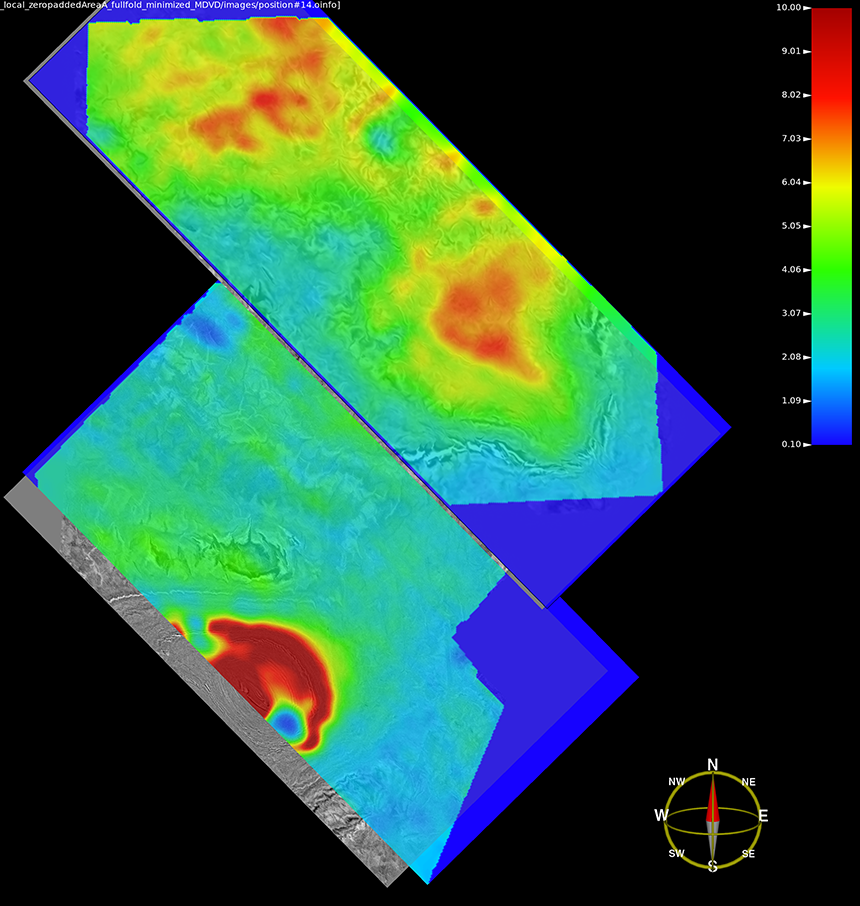~9000 sq. km horizontal resistivity depth image from the Barents Sea