

Quantum computers exploit the peculiar behavior of objects at the atomic scale and use the ‘qubit’ as the basic unit of quantum computing. A quantum computer with only 100 qubits would, theoretically, be more powerful than all the supercomputers on the planet combined, and a few hundred qubits could perform more calculations instantaneously than there are atoms in the known universe. A computer with 79 qubits has already been built.
In this article, after discussing one of the most popular methods to build qubits, PGS Chief Scientist and technology commentator Andrew Long then addresses the critical phenomena of superposition, entanglement and interference that allow quantum circuits built from qubits to be so powerful. Consideration is given to one possible way of building qubits with superconducting circuits, and how such devices may be programmed. A notable feature is that quantum algorithms work not by the use of brute force, but by exploiting underlying patterns that can only be seen from a quantum viewpoint. An apparent application to the oil industry is the potential for machine learning solutions to work with far deeper levels of data complexity.
From Classical Computers to Quantum Computers
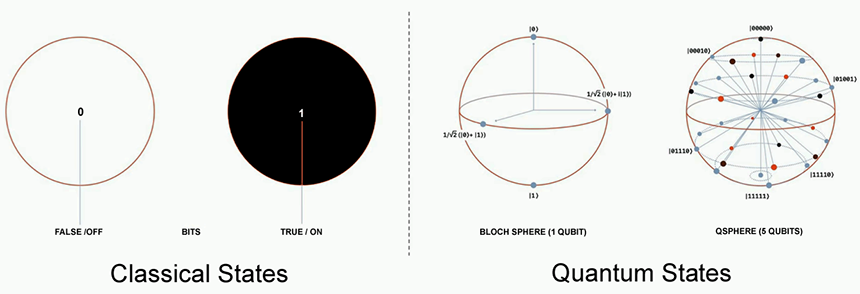
At the smallest scale, traditional microprocessor chips use logic gates built from transistors that perform instructions in terms of bits having discrete values of 0 or 1, the only two possible states. The standard example is an electrical switch (such as a transistor) that can be either on or off. Around 50 billion transistors can be accommodated on the most sophisticated chips, each having sizes as small as about 5 nm. This is getting close to the physical limits of engineering, so growth in computational power is achieved by building massive arrays of multi-processor chips; with the largest supercomputers today being capable of executing more than 100-quadrillion (100 x 1015) floating-point operations per second; otherwise referred to as 100 petaflops (PFLOPs).
The basic unit of quantum computing is the quantum bit, or ‘qubit’. This can be represented, for example, by the spin of an electron or the polarization of a photon, but the properties of spin and polarization are not nearly as familiar as a switch in the on or off position.
Quantum computers exploit the peculiar behavior of objects at the atomic scale—notably two properties known as ‘superposition’ and ‘entanglement’. At the atomic scale, particles can exist ‘superposed’ in many states at once, and two particles can exhibit ‘entanglement’ so that changing the state of one may instantaneously affect the other—regardless of how far apart the entangled particles may be. Qubits exploit these properties, but as discussed below, qubits rapidly ‘decohere’, or lose their delicate quantum nature after several seconds, and are extremely sensitive to any form of light, heat or radiation inside the quantum computer.
A quantum computer with only 100 qubits would, theoretically, be more powerful than all the supercomputers on the planet combined, and a few hundred qubits could perform more calculations instantaneously than there are atoms in the known universe. Quantum computing power scales exponentially with qubits (i.e. N qubits = 2N bits). The largest quantum computer built so far is the 79 qubit facility built by IonQ. As discussed below, ‘quantum supremacy’ will be reached when quantum computers overtake traditional supercomputers.
How do you Build a Qubit?
Quantum Superposition
A qubit in its quantum state can take values of |0⟩ (sometimes called the ground state because it is the lowest energy state), |1⟩, or a linear combination of the two (superposition). The half angle bracket notation |⟩ is conventionally used to distinguish qubits from ordinary bits. When you measure the |0⟩ quantum state, you get a classical 0, and when you measure the |1⟩ quantum state, you get a classical 1. Together, |0⟩ and |1⟩ make up ‘standard basis vectors’, which like all vectors, point in a direction and have a magnitude.
Additionally, qubits also have a ‘phase’, which results from the fact that superpositions can be complex. The basis states |0⟩ and |1⟩ and their linear combinations a|0⟩ + b|1⟩ describe the state of a single qubit. Visualizing a qubit commonly uses the ‘Bloch Sphere (refer to Figure 1). The Bloch Sphere is a sphere with a radius of one and a point on its surface represents the state of a qubit. Points on the surface of the Bloch sphere which lie along the X, Y, or Z axis correspond to special qubit states. When the qubit is in a superposition of |0⟩ and |1⟩, the vector will point somewhere between |0⟩ (up) and |1⟩ (down), and rotations around the Z-axis indicate a change in the phase of the qubit.
In practice, a qubit can be any two-level quantum system that you can address using external controls. Two discrete quantum energy levels then serve as your quantum |0⟩ and |1⟩ state. Popular mechanisms for qubits include photons, electron spin, trapped ions, neutral atoms, and superconducting circuits (below).
Quantum Entanglement
At this point, we need to consider ‘quantum entanglement’, which is a phenomenon in which the quantum states of two or more objects have to be described with reference to each other, even though the individual objects may be spatially separated. In other words, if two quantum objects become entangled, a change in the state of one will be spontaneously observed in the state of the other object—irrespective of how far apart the objects are. One application has been so-called quantum teleportation—as demonstrated when the low-orbit Chinese satellite Micius connected independent single-qubits to a ground station 1400 km apart. Quantum entanglement is necessary for qubits to be combined in a quantum computer (below).
Various physical processes can create entanglement—the most commonly used method today involving photons. A laser beam sends photons through a special crystal. Most of the photons just pass through, but some photons split into two. Energy and momentum must be preserved—the total energy and momentum of the two resulting photons must equal the energy and momentum of the initial photon. The conservation laws guarantee that the state describing the polarization of the two photons is entangled.
In the case of electron spin, it is possible to prepare two particles in a single quantum state such that when one is observed to be spin-up, the other one will always be observed to be spin-down and vice versa. The main problem with using entangled electrons that are near one another and then separating them is that they have a tendency to interact with the environment. On the other hand, photons are much easier to separate, though more difficult to measure.
The IBM Version of a Quantum Computer
The preference by IBM and Google for building entangled qubits is specially engineered superconducting circuits. IBM’s quantum computer considered below uses superconducting circuits built from Niobium (Nb) and Aluminum (Al) on silicon wafer circuits in which two distinct electromagnetic energy states make up a qubit. This approach has several key advantages. The hardware can be made using well-established manufacturing methods, and a conventional computer can be used to control the system. The qubits in a superconducting circuit are also easier to manipulate and less delicate than individual photons or ions.
The electrons in a superconductor pair up, forming what are called ‘Cooper pairs’. These pairs of electrons act like individual particles. The relevant fact is that the energy levels of the Cooper pairs in a superconducting loop that contains a ‘Josephson junction’ are discrete and can be used to encode qubits (refer to Figure 2). A qubit of this type is essentially a nonlinear LC resonator—a linear capacitor and a nonlinear inductor connected in series. The inductor is the Josephson junction—a pair of superconducting Aluminum electrodes that are separated by a very thin insulator that is a thousandth of a hair thick. The Josephson junction creates the nonlinearity that enables the LC resonator to act as an artificial atom with two quantum energy levels: |0⟩ and |1⟩. In other words, the energy level can be modeled as a quantum harmonic oscillator with quantized energy level. Without the non-linear element of the Josephson junction, the energy levels are equally spaced and less easily controlled.

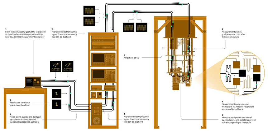
IBM’s quantum chips contain qubits made in a pattern generated with electron-beam lithography. Microwave buses tie the qubits together to make a qubit processor, and an input/output is provided by coupling the qubit to a superconducting transmission line resonator. The qubit transition frequency depends on the capacitances and inductances in the qubit circuit. Quantum operations are performed by sending electromagnetic impulses at microwave frequencies (around 4–6 KHz) to the resonator coupled to the qubit. This frequency resonates with the energy separation between the energy levels for |0⟩ and |1⟩. These calibrated microwave pulses correspondingly put qubits into superposition, and similarly, other frequencies and durations of these pulses can flip the qubit so that it’s in a slightly different state (but still in superposition). Furthermore, applying microwave pulses between a pair of qubits entangles them so that they always exist in the same quantum state. Because of the predictive nature of entanglement, adding qubits exponentially explodes a quantum computer’s computing power. To determine the result of a qubit’s operation, a measurement signal is sent as a microwave pulse to the qubit’s resonator. The measurement destroys the qubit’s superposition and collapses the qubit’s state to 0 or 1. Finally, interference allows scientists to control states to amplify the type of signals towards the right answer and cancel those leading to wrong answers. Scientists often have to run a problem multiple times to double-check the answer.
Each quantum processor rests at the bottom of a large dilution refrigerator where the temperature is kept below 15 milliKelvins—just above absolute zero and colder than the vacuum of space (Figure 3). This elaborate device is necessary because the quantum states of the qubits in the processor are extremely delicate. The slightest external disturbance—including heat, vibration and electromagnetic radiation—will destroy the quantum states in a process known as decoherence. What was once a physicist’s dream is now an engineer’s nightmare. Microwaves that carry control and measurement signals to the quantum chip are transmitted through coaxial cables. As the pulses travel through each of the refrigerator’s stages, they pass through attenuators to ensure thermal noise does not reach the processor. The reflected signal travels back up the dilution refrigerator, passing through isolators that protect the qubits from noise as well as amplifiers that boost the signal’s strength enough to read the qubit’s state accurately. The signal then passes back through the stack of microwave electronics, this time to be converted from microwave frequency to a digital signal that is sent over the internet to the local computer to display the result of the quantum calculation.
Programming a Quantum Computer
All computations whether classical or quantum in nature involve inputting data, manipulating it according to certain rules, and then outputting the final answer. Quantum gates and circuits are a natural extension of both classical gates and circuits. A classical logic gate (built with an interconnected array of transistors) gets a simple set of inputs and produces one definite output. A quantum gate or quantum logic gate is a rudimentary quantum circuit operating on a small number of qubits, and that changes the state of the qubits. Quantum logic gates are reversible, unlike many classical logic gates. Other universal classical logic gates, such as the Toffoli gate, provide reversibility and can be directly mapped onto quantum logic gates.
The quantum programming goal is to encode parts of a problem into a complex quantum state using qubits, and then apply quantum gates to entangle them and manipulate probabilities (the various superpositions), and finally measure the outcome, collapsing superpositions to an actual sequence of 0s and 1s. What this means is that the entire set of calculations that are possible with each setup are done at the same time. As with classical programming, scientists are now working to move low-level assembly languages, which the machine better understands, to high-level languages and graphical interfaces more suited for the human mind.
In 2016 IBM connected a small 5-bit quantum computer to the cloud. A programming toolkit called QISkit lets experimenters set up problems and drag-and-drop logic gates, thereby enabling simple programs to be written by anyone.
Applications for Quantum Computers
Popular descriptions of quantum algorithms describe them as being much faster than regular algorithms, but not every algorithm is susceptible to a quantum speedup. The algorithms work not by the use of brute force, but by ways of exploiting underlying patterns that can only be seen from a quantum viewpoint.
As noted, quantum theory predicts that a computer with N qubits can exist in a superposition of all 2N of its distinct logical states. This is exponentially more than a classical linear superposition. Note that though superposition is stronger than probabilism, it is weaker than actually having an army of 2N real computers all working on the problem at once. Superposition is strictly weaker than full parallelism and strictly stronger than probabilism.
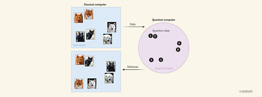
In the short term, quantum computers are being used to simulate and understand complex chemical processes and material properties down to the atomic level, take cryptography and digital security to new dimensions or supercharge artificial intelligence by crunching data more efficiently. Notably, machine learning could potentially process complex problems beyond current abilities at a fraction of the time, and therein lies potential applications to the oil industry. The study by Havlíček et al. (2019) published in Nature used a two-qubit quantum computing system to show that quantum computers can bolster a specific type of machine learning—one generally used for classification—by exploiting higher dimensionality feature spaces. As noisy as they are, the quantum systems already available seem functional—particularly those that can synergize with classical computers to perform machine learning as a team.
Bill Gates observed more than 20 years ago that the industry tends to overestimate the change that will occur in the next two years and underestimate the change that will occur in the next ten. AI and Big Data also require vast amounts of data storage in addition to harnessing computing power, so there are several things to consider, but the unique perspectives enabled by quantum computing make it definitely an emerging technology to watch.
References
Google AI Quantum https://ai.google/research/teams/applied-science/quantum-ai/
Havlíček, V., Córcoles, A.D., Temme, K., Harrow, A.W., Kandala, A., Chow, J.M., and Gambetta, J.M., 2019, Supervised learning with quantum-enhanced feature spaces. Nature, 567, 209–212. https://www.nature.com/articles/s41586-019-0980-2
IBM Q Experience https://quantum-computing.ibm.com/login
IonQ Trapped Ion Quantum Computing https://ionq.co/
Quantum Computing: you know it’s cool, now find out how it works https://www.ibm.com/blogs/research/2017/09/qc-how-it-works/
Quantum Machine Learning https://en.wikipedia.org/wiki/Quantum_machine_learning
Ren, J.-G., et al. (32 authors), 2017, Ground-to-satellite quantum teleportation. Nature, 549, 70-73. https://www.nature.com/articles/nature23675
Wiebe, N., Kapoor, A., and Svore, K., 2015, Quantum algorithms for nearest-neighbor methods for supervised and unsupervised learning. Quantum Information & Computation, 15(3 & 4), 318-358. https://arxiv.org/abs/1401.2142v2
Contact a PGS expert
If you have questions related to our business please send us an email.